Soft constraints penalty
Soft constraints are used to generate a penalty function. There are two general categories of penalty functions: linear distance and exponential. Within each of these categories there are several sub-categories. It is important to understand their behavior since poor selection can ruin the optimization.
Linear Distance Penalty = (Portfolio Value – Target Value) / Target Value
Note that if penalties occur in more than one period they are added. This means that a small deviation over many time periods will generate a large penalty. This result may be desired or not depending on the circumstances.
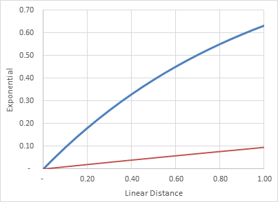
Exponential Penalty = 1 – EXP ( - Linear Distance Penalty / 10 )
The inclusion of the divisor of 10 is designed to make the penalties more useful as the overall penalties will not be so big that they will wash out potentially viable portfolios.
The total penalty is calculated as the average of all periods instead of the sum.

The chart above shows the relationship between exponential and linear distance (blue) with the
Choosing which to use depends on your view on outliers. For example, perhaps it doesn’t matter if the production target is missed badly in one year as long as it is close in most years (use exponential). Conversely it may be critical that a capex constraint is met every year and there is no option to massively exceed it in one year (use linear distance).
Time Weighted (TW) The penalty is reduced for later periods. It is discounted in each period according to its weight (5% or 25%). This can be selected to ensure that most focus is placed on the first years and less on later periods.
Soft Threshold (ST) The threshold sets a cap on the maximum penalty for a given period. If the penalty exceeds 30%, it will be set to 30% for that period. This reduces the impact of large outliers in a given period on the total penalty.
Hard Threshold (HT) The threshold sets a cap on the maximum penalty for a given period. If the penalty exceeds 100%, it will be set to 100% for that period. This reduces the impact of large outliers in a given period on the total penalty.
Here is a numerical example of the penalty functions that would result for some sample data:
| 2014 | 2015 | 2016 | 2017 | 2018 | 2019 | Total | Average | |
|---|---|---|---|---|---|---|---|---|
| Target | 120 | 120 | 120 | 120 | 120 | 120 | ||
| Portfolio Value | 80 | 90 | 102 | 112 | 122 | 132 | ||
| Linear Distance Penalty | 0.33 | 0.25 | 0.15 | 0.07 | - | - | 0.800 | |
| TW05 discount | 1.00 | 0.95 | 0.91 | 0.86 | 0.82 | 0.78 | ||
| TW05 penalty | 0.33 | 0.24 | 0.14 | 0.06 | - | - | 0.765 | |
| TW25 discount | 1.00 | 0.80 | 0.64 | 0.51 | 0.41 | 0.33 | ||
| TW25 penalty | 0.33 | 0.20 | 0.10 | 0.03 | - | - | 0.663 | |
| Soft Threshold ST30 | 0.30 | 0.25 | 0.15 | 0.07 | - | - | 0.767 | |
| Exponential Penalty | 0.03 | 0.02 | 0.01 | 0.01 | - | - | 0.013 | |
| TW05 penalty | 0.03 | 0.02 | 0.01 | 0.01 | - | - | 0.076 | |
| TW25 penalty | 0.03 | 0.02 | 0.01 | 0.00 | - | - | 0.065 |